> For the complete documentation index, see [llms.txt](https://blogs.labii.com/llms.txt). Markdown versions of documentation pages are available by appending `.md` to page URLs; this page is available as [Markdown](https://blogs.labii.com/feature-updates/2019-08-26-elisa-standard-curve-with-labii-eln-and-lims-in-3-steps.md).
# 2019-08-26 ELISA Standard Curve With Labii ELN & LIMS In 3 Steps
[ELISA](https://www.thermofisher.com/us/en/home/life-science/protein-biology/protein-biology-learning-center/protein-biology-resource-library/pierce-protein-methods/overview-elisa.html) (enzyme-linked immunosorbent assay) is a plate-based assay technique designed for detecting and quantifying substances such as peptides, proteins, antibodies and hormones. In an ELISA, an antigen must be immobilized on a solid surface and then complexed with an antibody that is linked to an enzyme. Detection is accomplished by assessing the conjugated enzyme activity via incubation with a substrate to produce a measurable product. The most crucial element of the detection strategy is a highly specific antibody-antigen interaction.\
\
After an ELISA has been run, the data must be analyzed. The ELISA data analysis requires many different steps but it is still relatively simple compared to deep sequencing data analysis. The lack of market profit leads to limited solutions available. [Excel](https://www.mdbioproducts.com/resources/protocols/standard-curve) and Graphpad are the two most used solutions.\
\
The [scatter chart ](https://www.mdbioproducts.com/resources/protocols/standard-curve)is used to generate a standard curve in Excel. It usually takes around 15 steps to get the analysis results for one 96-well plate. Similarly, the scatter chart is also used when [analyzing ELISA data with Graphpad](https://www.graphpad.com/support/faq/graphpad-tutorials-elisa-analysis-with-prism/). Before getting started with Graphpad, the data must be prepared and normalized in an excel sheet. The data can then copied to the GraphPad and use XY scatter chart.\
\
Overall, the problem of the current methods are 1) they are tedious and requires 15-20 steps to finish the analysis to one 96-well plate; 2) easy to make mistakes - for all the manual steps involved, any single mistake involved by human will result in unspotted mistakes in the final results; 3) it is difficult to document the process - the data generated in biotech and pharmaceutical companies usually required to meet the regulatory requirements of FDA 21 CFR part 11. The manual steps make it very difficult to record all the processes.\
\
To resolve such problem and make the data analysis of ELISA data more straightforward, [Labii](https://www.labii.com/) has developed a widget to perform the ELISA data analysis directly in the [Electronic Lab Notebook (ELN)](https://www.labii.com/electronic-lab-notebook-eln) platform. [The widgets at Labii ELN & LIMS is a stand-alone function to edit or process a certain piece of data](https://docs.labii.com/widgets/summary). We first create the layout of the 96-well plate for both layout and data, then we automatic all 15 steps at either Excel or Graphpad into one simple click. The widget can be [inserted into experiments](https://docs.labii.com/quick-start) just like all other widgets. [The detail documentation about the ELISA data analysis widget can be found here](https://docs.labii.com/widgets/biology/elisa-standard-curve).\
\
Here, I will show you how to perform ELISA data analysis with Labii [Electronic Lab Notebook (ELN)](https://www.labii.com/electronic-lab-notebook-eln) and [Laboratory Information Management System (LIMS)](https://www.labii.com/laboratory-information-management-system-lims) in 3 steps:
## **Step 1: Prepare layout**
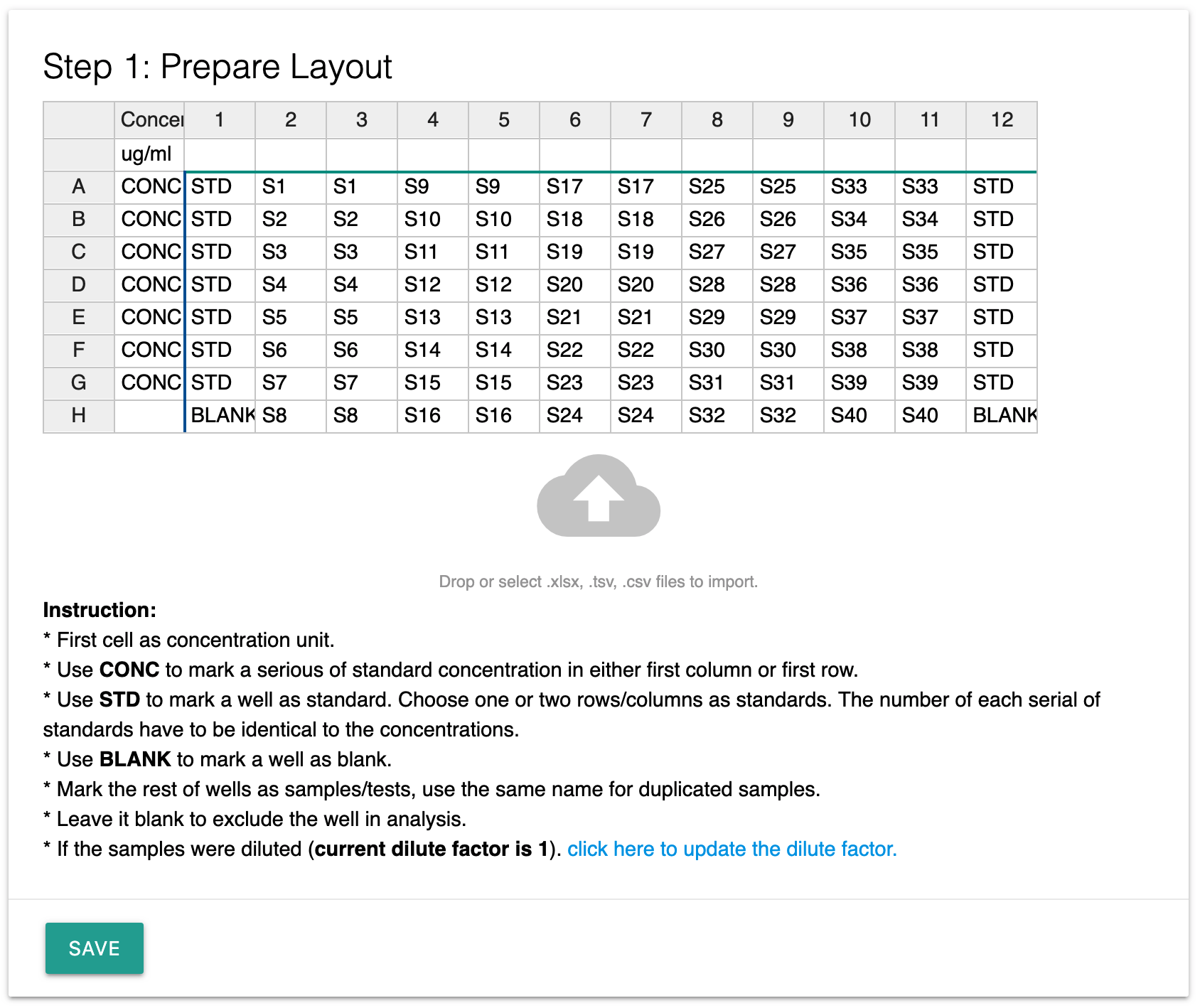
Once you added the widget, you can prepare the ELISA layout by typing or import the data directly from your excel file. You can do so by dragging an excel file into the cloud area.
Prepare ELISA Layout
To enable the widget to recognize the data, please keep in mind:
1. Use the first cell as the concentration unit. For example ug/ml.
2. Use CONC to mark a serious of standard concentration in either the first column or first row.
3. Use STD to mark a well as standard.
4. Use BLANK to mark a well as blank.
5. The same name is treated as duplicates.
6. Leave a well blank to exclude the data point in the analysis.
Please also follow these [good practices](https://www.thermofisher.com/us/en/home/life-science/protein-biology/protein-biology-learning-center/protein-biology-resource-library/pierce-protein-methods/overview-elisa/elisa-data-analysis.html) to generate valid persuasive ELISA results:
1. **Run samples in replicate.** To help evaluate the extent of error, each standard and sample should be tested in replicate (duplicate or triplicate, depending on the number of samples and room on the plate). Afterward, the average, standard deviation (SD), and coefficient of variation (CV) can be calculated to provide confidence in pipetting precision. As a best practice, the replicates should have a CV of less than 20%. If the CV is higher than 20%, consider the following (Reasons the CV may be high):
1. Pipetting errors—Check pipetting technique. See the ELISA Troubleshooting Guide for proper pipetting techniques.
2. Contamination of plates or reagents—Make sure plates and reagents are stored properly and don’t get cross-contaminated. Also, check reagents for expiration dates.
3. Temperature across plate—Incubate plates in a stable environment to ensure even temperature.
4. Evaporation—Use plate covers during all incubation steps.
2. **Run a standard curve on every plate.** Every ELISA runs slightly differently depending on the operator, pipetting, incubations, and temperature. Taking these variables into account, it is a best practice to run a standard curve on each plate.
3. **Run a positive control sample.** Running a control sample with a known concentration on each plate will indicate whether the ELISA was successfully executed. If the control sample represents the correct concentration, you can be confident in the results of the other unknown samples.
4. **Run blank samples.** Blank samples are composed of the buffer or water with no protein sample included. These samples allow the subtraction of background absorbance from the rest of the data points to ensure the most accurate OD readings.
5. **Dilute samples so they fall within the linear range of the standard curve.** To get the most accurate results, dilute the samples so they fall within the linear range of the standard curve. Values that fall toward the top or bottom of the curve tend to have a higher amount of error because of the assay’s limits. Many operators test samples at multiple dilutions to ensure that at least one of them falls within the linear range.
## **Step 2: Prepare data**
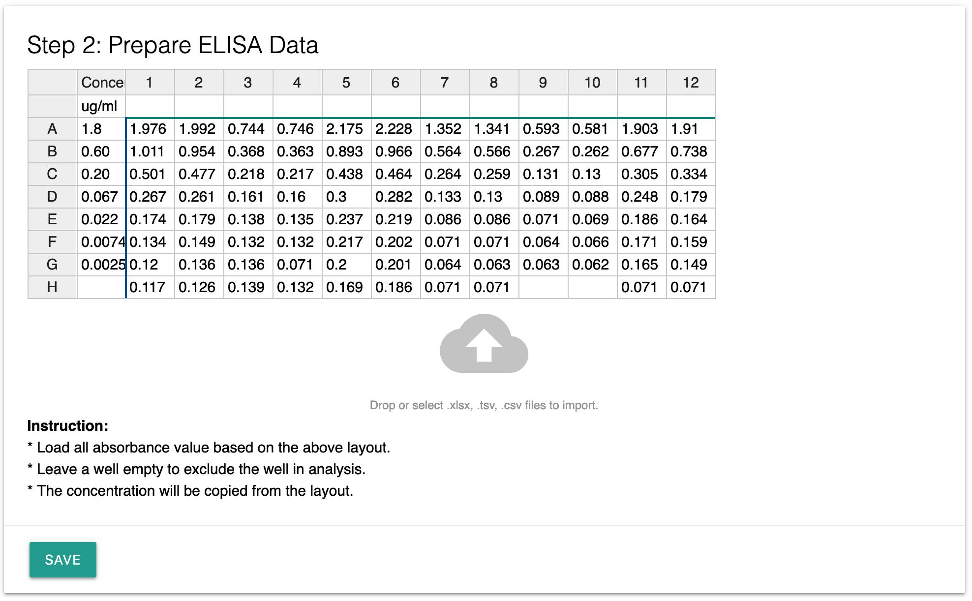
Compare to data preparation in Excel and Graphpad, the data preparation in [Labii](https://www.labii.com/) is much simpler. Just drag the file over the cloud icon and all ELISA data will be load automatically.
Prepare ELISA Data
## **Step 3: Perform the analysis**
Once the data is ready, to perform the ELISA data analysis is as simple as a click. Click the Analysis button and the analysis will start right away. All results will be included in the analysis section once finished. The analysis only takes a few seconds.\
\
Here are the details about the analysis:\
\
1\. Generate the average absorbance of blanks\
Labii will use the layout you created at step 1 to find all blank wells. The average value will be calculated and displayed back to you.
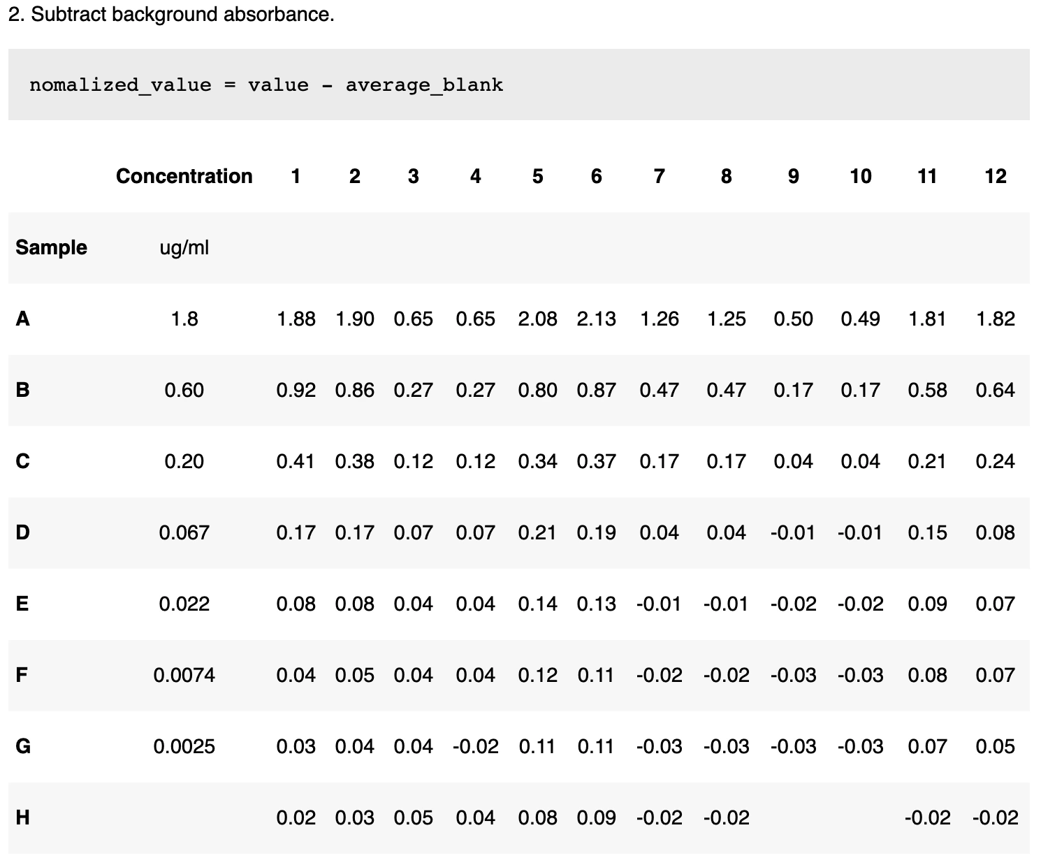
2\. Subtract background absorbance\
The normalized value for all data points is calculated via subtracting the background absorbance (the average value of the blanks). If the blank samples are reading higher than usual, this may indicate that there was an error in the assay.
3\. Generate the average absorbance of the standard\
If multiple standards are used, the absorbance of the standard at the same concentration will be calculated. This value will be used in plotting and fitting.\
\
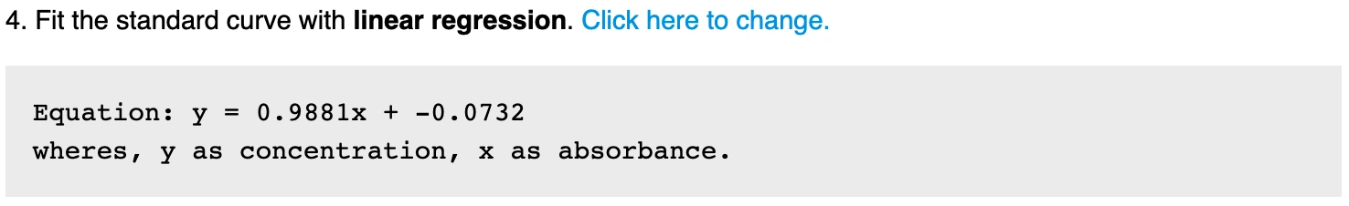
4\. Fit the standard absorbance\
On default, [Labii electronic lab notebook](https://www.labii.com/electronic-lab-notebook-eln) uses linear regression to fit the standard absorbance with the standard concentrations. Labii also provide you the option to use other regression methods. You can click the edit icon to change the repression method:
* linear - Fits the input data to a straight line with the equation `y = mx + c`.
* exponential - Fits the input data to an exponential curve with the equation `y = ae^bx`.
* logarithmic - Fits the input data to a logarithmic curve with the equation `y = a + b ln x`.
* power - Fits the input data to a power law curve with the equation `y = ax^b`.
* polynomial - Fits the input data to a polynomial curve with the equation `anx^n ... + a1x + a0`.
Once it is finished, the fit equation will be generated and displayed for references. The calculated standard point will be used for plotting.
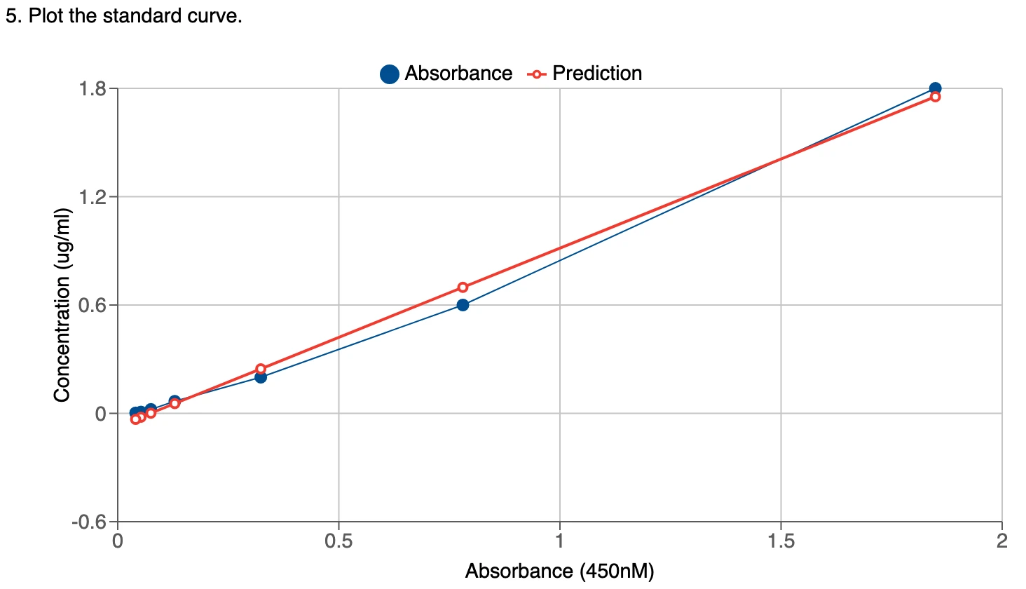
5\. Plot standard curve\
A standard curve for the target protein by plotting the mean absorbance (y-axis) against the protein concentration (x-axis). A best-fit curve through the points in the graph will also be added based on the calculated value from fitting.
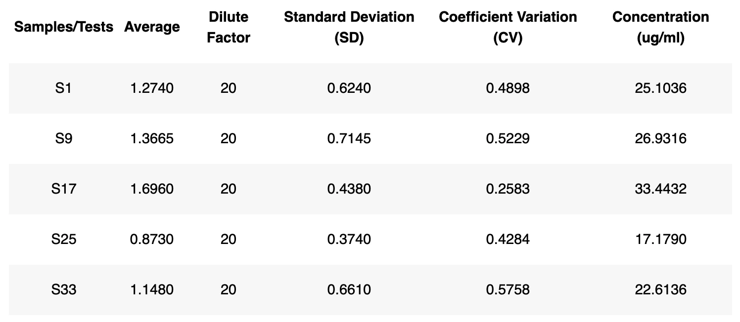
6\. Calculate SD, CV, and concentration
* **Concentration** - The mean value of a sample/test/project will first generate. This mean value will then used in the fitting model to calculate the corresponding concentration. The final concentration will be multiple the dilution factor.
* **Standard Deviation (SD)** - The standard deviation is a measure that is used to quantify the amount of variation or dispersion of a set of data values. The SD will be calculated for each sample.
* **Coefficient Variation (CV)** - The coefficient variation (CV) is the ratio of the standard deviation σ to the mean µ: Cv= σ / µ. This is expressed as a percentage of variance to the mean and indicates any inconsistencies and inaccuracies in the results. Larger variance indicates greater inconsistency and error. Labii calculates the CV values for each sample.\
Once done, the sample, average value, SD, CV, and concentration will be displayed in a table. You can click the table header to sort the table.\
## **Summary**
With Labii's ELISA Data Analysis widget, you can document and analyze the data in a few clicks, and the result is ready in a few seconds. Labii's ELISA Data Analysis widget is flexible and can meet all of your ELISA layout design. It also provides you multiple regression methods to meet your analysis for log files. Labii ELN & LIMS is the only [Electronic Lab Notebook (ELN)](https://www.labii.com/electronic-lab-notebook-eln) in the market that is able to provide this kind of applications. To learn more, schedule a meeting with Labii representatives ([https://call.skd.labii.com](https://call.skd.labii.com/)) or create an account () to try it out yourself.\
\
Yonggan Wu